DBCC SHOW_STATISTICS: A Deep Dive with Practical Examples

In this Article we describes the command step by step and demonstrates several actual examples. With such results, you will be able to optimize queries and performance.

“DBCC” The meaning of “DBCC” is Database Console Command. “SHOW_STATISTICS” request the order to show the system information about the statistics within indexes. The statistics of each index are on a table.

Understanding DBCC SHOW_STATISTICS

DBCC SHOW_STATISTICS displays optimizer statistics of the current query on a table or an indexed view. Query optimizer uses such statistics to determine the approximate number of rows a query will retrieve which is essential in selection of the most efficient execution plan. Obsolete statistics or out-of-date statistics may result in poor plans and poor query performance.
Its simple syntax is:
DBCC SHOW_STATISTICS ( table_name , target )
table_name: The indexed view or table's name.
target: _WA_Sys_<column_id>_<hex_id> for auto-generated statistics, or the name of the index or statistics. Statistics information for every statistic in the table is returned if the target is left out.

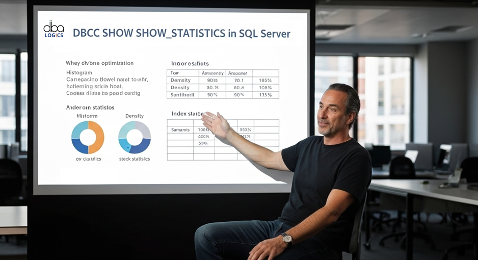
The result of DBCC SHOW_STATISTICS output is categorized in three ways:

Statistics Header: In Statistics header, the name of the object, last-updated date, number of rows, and number of rows sampled are mentioned.
Density Vector: Density vector indicates how the data values are unique. The more unusual the values are the denser the pattern is.
Histogram: The histogram of the leading column will indicate the range of values that there are and the number of rows contained in each range.

Examples

Let's consider a table named `Orders` with the following structure (simplified for clarity):

CREATE TABLE [dbo].[Orders](
    [Id] [int] NOT NULL,
    [CustomerId] [int] NOT NULL,
    [OrderDate] [smalldatetime] NOT NULL,
    [Amount] [int] NOT NULL,
    [Status] [tinyint] NOT NULL,
    [Other] [char](500) NOT NULL,
    [CustId] [varchar](20) NULL,
    [DeliveryDate] [smalldatetime] NULL
)

Let's populate the table with some sample data:
INSERT INTO Orders
    (Id, CustomerId, OrderDate, Amount, Status, Other, CustId, DeliveryDate)
VALUES
    (1, 364438, '2001-07-17', 7640, 1, 'abcd', 364438, '2000-06-14'),
    (2, 974915, '1999-08-22', 7230, 1, 'ABCD', 974915, '1998-07-18'),
    (3, 111172, '2004-03-27', 6381, 1, 'abcd', 111172, '2003-02-24'),
    (4, 522921, '1989-04-09', 101, 1, 'ABCD', 522921, '1988-03-07'),
    (5, 925726, '1988-06-06', 101, 1, 'abcd', 925726, '1987-05-06'),
    (6, 99778,  '2018-02-05', 2214, 1, 'ABCD', 99778,  '2016-12-31'),
    (7, 335251, '1998-06-02', 8059, 1, 'test', 335251, '1997-04-29'),
    (8, 5801,   '2015-09-03', 2725, 1, 'test', 577116, '2014-08-02'),
    (9, 670562, '2011-07-17', 6021, 1, 'test', 670562, '2010-06-17'),
    (10, 731364,'1997-11-14', 4025, 1, 'test', 731364, '1996-10-15');

Lets get data
--OutPut
Id          CustomerId  OrderDate               Amount      Status Other                          CustId               DeliveryDate
----------- ----------- ----------------------- ----------- ------ ------------------------------ -------------------- -----------------------
1           364438      2001-07-17 00:00:00     7640        1      abcd                           364438               2000-06-14 00:00:00
2           974915      1999-08-22 00:00:00     7230        1      ABCD                           974915               1998-07-18 00:00:00
3           111172      2004-03-27 00:00:00     6381        1      abcd                           111172               2003-02-24 00:00:00
4           522921      1989-04-09 00:00:00     101         1      ABCD                           522921               1988-03-07 00:00:00
5           925726      1988-06-06 00:00:00     101         1      abcd                           925726               1987-05-06 00:00:00
6           99778       2018-02-05 00:00:00     2214        1      ABCD                           99778                2016-12-31 00:00:00
7           335251      1998-06-02 00:00:00     8059        1      test                           335251               1997-04-29 00:00:00
8           5801        2015-09-03 00:00:00     2725        1      test                           577116               2014-08-02 00:00:00
9           670562      2011-07-17 00:00:00     6021        1      test                           670562               2010-06-17 00:00:00
10          731364      1997-11-14 00:00:00     4025        1      test                           731364               1996-10-15 00:00:00

  Let's populate the table index with some sample
CREATE INDEX IX_Orders_CustomerID ON Orders (CustomerID);
CREATE INDEX IX_Orders_OrderDate ON Orders (OrderDate);
Example 1: Examining Statistics on an Index

To view the statistics for the IX_Orders_CustomerID index, we can use the following command:

DBCC SHOW_STATISTICS (Orders, IX_Orders_CustomerID)
GO

 This report has three sections:
Statistics header
Rows: number of rows that the table contains (10, in this case)
Rows Sampled: the number of rows sampled, or number of rows less than the total when based on a sample and therefore less accurate;
in this case 0 (this data item was very low on our list during the test). Last updated- Indicates the date when the statistics were last time checked and updated
Density Vector
The value of the density is the reciprocal of the count of different values in the CustomerID column.
The smaller the value of density, the more sharp the values which is preferable.
In our example of 4 different CustomerID values (101, 102, 103, 104), density would be approx. 0.25.
Histogram
The occurrence of the CustomerID values is depicted in the histogram.
It takes the range of values and divides it into steps and indicates the number of rows that will lie within each step.

Example 2: Analysis of Auto-generated Statistics

SQL Server will automatically generate statistics on individual columns when it deems this to be appropriate. These statistics are called such a name as _WA_Sys_ In order to view the statistics that have been generated against the Amount column you must identify the name of the auto generated statistic.

This name may be found by the following query:
SELECT a.name
FROM sys.stats a
WHERE a.object_id = OBJECT_ID('Orders') AND a.name LIKE '_WA_Sys_%'
AND STATS_ID in (SELECT STATS_ID FROM sys.stats_columns
WHERE object_id = OBJECT_ID('Orders')  AND column_id in (
SELECT column_id FROM sys.columns  WHERE object_id = OBJECT_ID('Orders')
AND name = 'Amount' ) );

Let's assume the query returns the name __WA_Sys_00000004_66EA454A. Then, you can view the statistics using:
DBCC SHOW_STATISTICS (Orders, '_WA_Sys_00000004_66EA454A');
GO

The graph will resemble the above one, although it will contain only amounts. In every bar there will be indicated the number of data rows that contain such amount.

Example 3: Impact of Outdated Statistics

Assuming that we add a huge number of new orders to a new customer (e.g., CustomerID = 105),

Statistics that exist become obsolete.

And going ahead, when we run a query like SELECT * FROM Orders WHERE CustomerID = 105, the query

optimizer may overestimate the number of rows which will be returned since the statistics

No longer reflecting the new data distribution. This may result in poor execution plan.

In order to correct that, we must refresh the statistics:

UPDATE STATISTICS Orders WITH FULLSCAN  

Once statistics are refreshed the query optimizer will have more correct knowledge of the manner that the data is distributed and can select a more efficient execution plan.

Conclusion:

DBCC SHOW_STATISTICS provides an excellent way of knowing the data distribution in tables and indexes. You may find out how the query optimizer works by examining the statistics header, density vector and histogram. It is also necessary to monitor and update statistics regularly in order to have optimal query performance. Always remember to update statistics whenever there are major changes of data so that it is updated to the query optimizer. WITH FULLSCAN is most precise in terms of statistics, but resource high-cost on large tables. You may also wish to use WITH SAMPLE to update quicker, though quite possibly not as accurately.